Expansion and Automation of the Unified Import System for Composite Skulls in OrtogOnBlender XP
Abstract
This study addresses the expansion and automation of the unified composite skull import system within the free software OrtogOnBlender XP, focusing on orthognathic surgery planning and maxillofacial procedures. The primary objective of the work was to overcome structural limitations of previous versions by implementing a redundant modular architecture to mitigate critical scale and mirroring errors. Among the most important and interesting findings, a stark disparity was observed between the new artificial intelligence-driven pipeline (TotalSegmentator + MeshSegNet) and the legacy tool DentalSegmentator. The new workflow proved to be approximately 22 times more accurate than the old one, achieving a global accuracy per patient of 95.65% against a mere 4.35% for the previous method, while also processing data in half the time (~10 minutes versus ~20 minutes). Comparative tests between operating systems also revealed crucial performance and structural data. In a first raw execution, the automated alignment of intraoral models achieved ~93% accuracy under Linux and ~86% under Windows. After coding fine-tuning, the success rate jumped to the impressive benchmarks of 97.83% under Linux and 93.18% under Windows. However, under a global evaluation per patient, Linux proved to be about 3 times more effective against residual failures, presenting only 1 error across 23 exams (~95% success rate), compared to 3 failures out of 22 exams under Windows. The study concludes that while automation drastically reduces active working time, visual human validation remains an indispensable layer of security in the digital planning workflow.
Keywords: Composite skulls, OrtogOnBlender XP, Artificial intelligence, TotalSegmentator, MeshSegNet, Intraoral scan alignment, Open-source surgical planning
Introduction
Launched in 2017, OrtogOnBlender (OOB) has evolved over the years from a study tool into a surgical planning tool de facto utilized by surgeons across 37 countries and widely published in peer-reviewed journals, addressing not only, but primarily, procedures within the human facial region.
A year ago, the first version of the unified import system for composite skulls was implemented [Moraes_et_al_2025_f]. To ensure this milestone is preserved over time, it is important to explain the challenges of that period and how this approach represented major progress.
In the early days of OOB development in 2017, the primary challenge was converting DICOM files into 3D objects—moving from a sequence of images (voxel data) to a 3D mesh. This was achieved using DicomToMesh (https://github.com/eidelen/DicomToMesh) via a primitive interface inside Blender, where the user specified the tomography directory and the Hounsfield scale factors to be reconstructed. Initially, the data-filling process was manual, but an automated approach based on a tomograph database was later implemented [Moraes_et_al_2021_f]. Although it was a well-developed tool, implementing DicomToMesh across different operating systems via OOB caused compatibility issues, prompting the transition to a Python-based solution (VTK+SimpleITK), which required significantly less effort for system porting [Moraes_et_al_2021b_f].
These tools represented a breakthrough by centralizing the workflow within a single software package, eliminating the need for external applications such as InVesalius (https://invesalius.github.io/) or Slicer (https://www.slicer.org/), although OOB has maintained a script-level connection with the latter to this day. Nonetheless, even with these advances, the segmentation phase still demanded significant knowledge and effort from the user. Initially, an anatomical landmark-based mandibular segmentation tool was developed; while it functioned in a significant percentage of cases, it presented structural boundary limitations (often over-segmenting) and required manual placement of landmarks, which could serve beginner users but was ignored by advanced ones who opted for manual segmentation, judging it more practical.
For replacing tomography teeth with intraoral scans (IOS), the process was simpler and more practical. Given that tomography segmentation occurred in three stages—the face, the skull, and the teeth (the densest part of the bone)—a lateral clipping tool was implemented so users could manually isolate the dental region for subsequent IOS alignment.
Porting external tools like computed tomography reconstruction and implementing specific commands using the Blender Python API (bpy) represented a major evolution and simplification of the surgical planning process. Although much of it still required manual user intervention, it became possible to develop a complete orthognathic surgery planning protocol within a single graphical interface based on free and open-source software [Moraes_et_al_2020_f].
In addition to anatomical reconstruction, cephalometry—including both Arnett and USP analyses—has been a core feature of OOB for several years. Facial structure projection for both soft tissue and the face is a native OOB solution that was published in a peer-reviewed journal [Abdullah_et_al_2022_f], received data updates from diverse populations [Moraes_and_Suharschi_2022_f], and was ultimately converted into a standard tool within the add-on.
Regarding artificial intelligence, the first tool developed focused on tooth segmentation in IOS models using MeshSegNet (https://github.com/Tai-Hsien/MeshSegNet), which was incorporated into the core of OOB [Moraes_and_Dakir_2021_f]. Subsequently, a multiple-component solution was tested, which aligned the tomography to the Frankfurt plane, positioned a series of anatomical landmarks, and automatically segmented various anatomical structures, such as the mandible and airways. Although highly dependent on Slicer, the tool was executed directly through OOB by simply indicating the storage directory of the DICOM files [Moraes_et_al_2024_f].
With the advent of OrtogOnBlender XP, built upon Blender 4.2, the tomography import system received user interface improvements and underwent a rigorous testing pipeline involving more than 400 tomographies, increasing its success rate from 96.78% to 100% [Moraes_et_al_2024b_f]. Immediately following this, an AI-driven tomography segmentation system was developed as a complementary and redundant layer to the previously created automatic framework. A new round of testing involved 151 tomographies with a 100% success rate [Moraes_et_al_2024c_f].
These two tools enabled the development of the unified composite skull system, allowing users to automatically import the tomography, perform AI-based segmentation, position a series of anatomical landmarks, and import and pre-align intraoral models. During this phase, 120 tests were performed on the unified system (excluding dental alignment), followed by 36 complete tests—12 within each operating system configuration (Linux, WSL, and Windows)—revealing a slight performance advantage for Linux [Moraes_et_al_2025_f]. In total, prior to the writing of this document, OOB XP had already accumulated 1,028 tool tests.
Although the unified system presented a major advancement, it still had structural limitations, such as the lack of individual tooth segmentation, an intraoral model alignment without guaranteed precision adjustment, an absence of anatomical measurement data, and a lack of pre-configured cephalometry tools.
The Framework Update
The unified composite skull generation system in OOB XP received some adjustments and optimizations without altering its previous core functionality, merely adapting the code to accommodate new technology insertions. This, in turn, generated a positive framework of complementary workflow options, enriching the add-on and granting the user greater flexibility and alternatives should any specific tool encounter an issue.
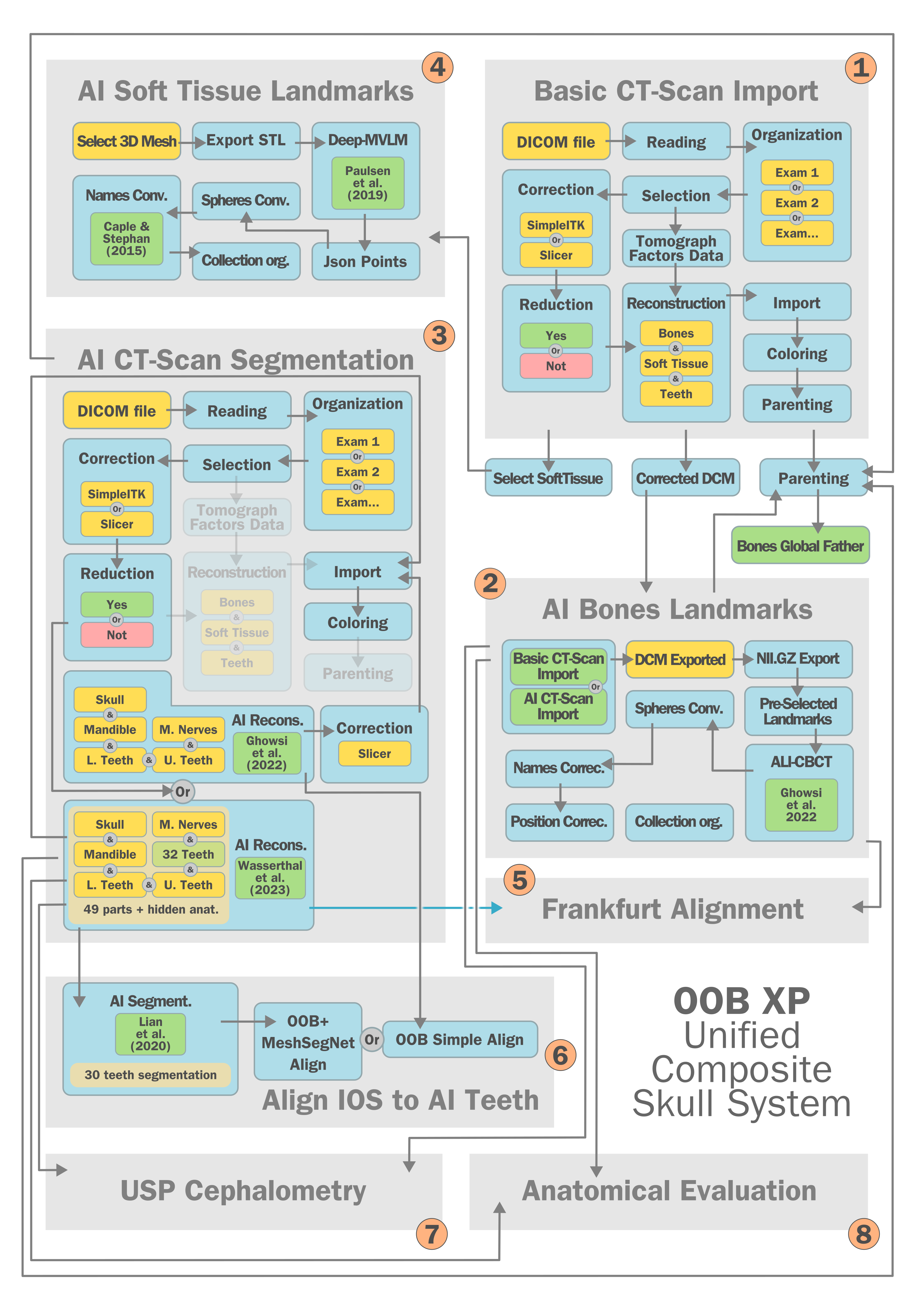
Fig. 53 Visual scheme of the unified composite skull generation system.
The current configuration of the system operates as follows:
0) The user specifies the directories containing the computed tomography scan files and the upper and lower scanned intraoral models (IOS).
1) A 3D reconstruction of the tomography is performed using the raw DICOM data based on the tomograph model database, outputting three distinct meshes: Bones, SoftTissue, and Teeth. The Bones mesh acts as the root in the parenting hierarchy, a structure reflected throughout subsequent processes; thus, the Bones mesh serves as the global standard of reference. This approach was chosen due to its historical reliability established through extensive testing and practical clinical use, making it the most robust tool developed among the others. Furthermore, keeping the primary structure intact provides an extra pre-operative reference, and the SoftTissue mesh—in the absence of an external photogrammetry scan—serves as the baseline for anatomical landmark placement and osteotomy-driven structural adjustments (Fig. 53, 1).
2) Next, the automated bone anatomical landmark positioning system via artificial intelligence is triggered. This system is fully independent and provides the necessary data to align the head to the Frankfurt plane, while offering references for the initial automatic positioning of osteotomies. It subsequently helps limit the zones of influence for facial adjustments during osteotomies, as well as assisting in facial measurements and cephalometric analysis (Fig. 53, 2).
3) Significant improvements were introduced in this phase, as the previous version already provided an anatomical segmentation, but practical usage tests revealed that the results on Windows were slightly inferior to those on Linux, processing times could extend excessively, and the system lacked individual tooth segmentation—a frequent user request. To address this, a system based on TotalSegmentator (https://github.com/wasserth/totalsegmentator) was implemented, building upon the work of [Wasserthal_et_al_2023_f]. When compared directly to the DentalSegmentator, this new pipeline reduced processing time by practically half, while delivering a significantly larger number of segmented anatomical pieces. This code integration enabled significant improvements in the IOS alignment system, as the software now computes teeth individually and works in tandem with MeshSegNet. It also provides complementary data for the Frankfurt alignment, as will be seen below (Fig. 53, 3). The detailed data regarding this time and accuracy comparison are presented later in the Testing and Best Practices section.
4) The SoftTissue mesh, which in practice is the “face”, receives a series of automated anatomical landmarks via artificial intelligence. These points provide spatial references for several subsequent approaches, such as boundary mapping for osteotomy influence zones, facial measurements, and cephalometric plotting (Arnett) (Fig. 53, 4).
5) OOB XP utilizes the anatomical landmark data generated primarily by Step 2 and complementarily by Step 3 to align the head along the Frankfurt plane. While not a unanimous choice among specialists—as some prefer the natural head position—it remains a widely documented and utilized orientation standard (Fig. 53, 5).
6) Another major upgrade occurs at this stage. The previous version (OOB Simple Align) provided a preliminary IOS alignment with a success rate of ~5% (only 1 in 20 cases resulted in full alignment). The new version inverted the logic and substantially improved system reliability; now, only 1 in 15 cases on Windows, or 1 in 46 on Linux, may present an alignment issue, boosting the success rate to a milestone of 93.18%–97.83%. This breakthrough was achieved by adapting MeshSegNet to the current Python version, cross-referencing data with anatomical landmarks derived from TotalSegmentator meshes, and implementing complementary programming within OOB itself (Fig. 53, 6). The cited numbers will be explained later in Tests and Best Practices.
7) The USP cephalometry system was successfully ported from OOB 2.9.1 to OOB XP. However, since anatomical landmarks are now positioned automatically, the current version generates a report immediately following the finalization of the unified composite skull generation process (Fig. 53, 7). Arnett cephalometry is also currently being ported.
8) The final stage consists of gathering anatomical measurements based on both population means and calculated proportions. This step also generates a color-coded statistical report of the results based on standard deviations (Fig. 53, 8).
How It Works
In the following sequence, a step-by-step guide will be provided for generating a composite skull using the most current approach of the tool.
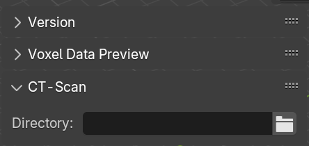
Fig. 54 CT-Scan section.
Initially, it is necessary to expand the CT-Scan section of OOB XP (available starting from version 2026-06-29). There, the directory selection must be performed. To do so, simply click on the directory icon at the bottom right (Fig. 54).
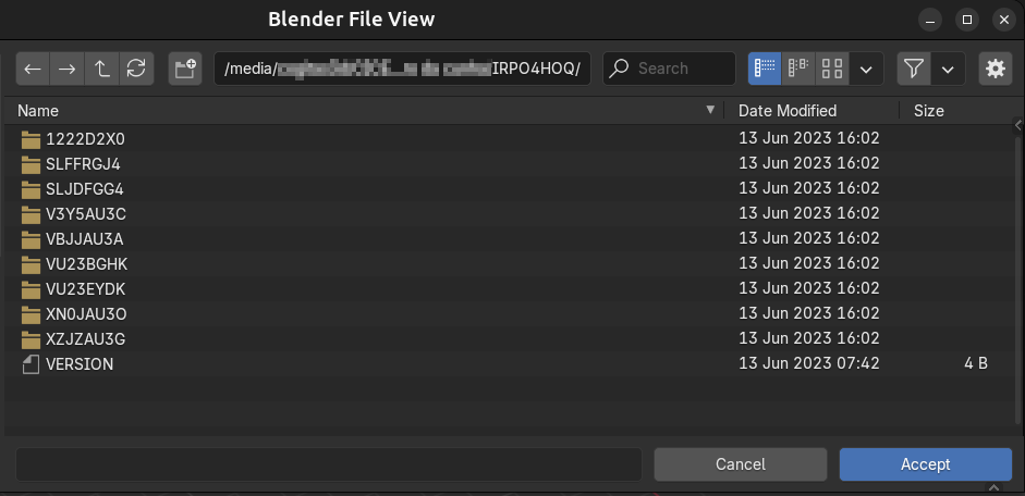
Fig. 55 Selection of the computed tomography root directory.
The next step consists of entering the root directory of the computed tomography scan. There is no need to select one of multiple folders, as OOB features a tomographic exam organization tool. That is, once in the root directory, simply click on Accept (Fig. 55).
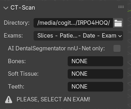
Fig. 56 Exam selector activated.
Once this is done, the exam selector is activated in Exams (Fig. 56).
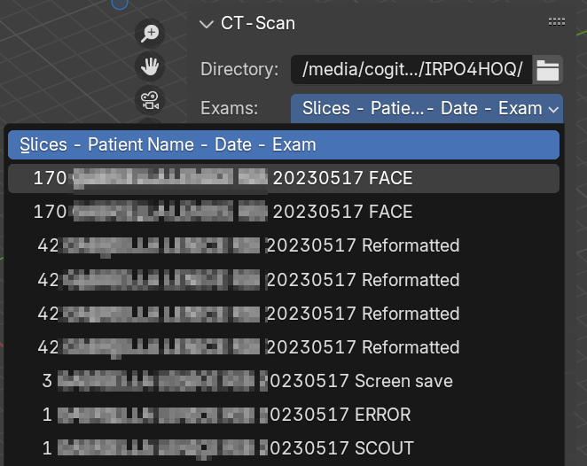
Fig. 57 Selection of the exam to be reconstructed in 3D.
By clicking on the menu, the user can select the exam they wish to reconstruct in 3D. The exams with the largest number of slices are presented at the top of the menu, with the following data sequence: Slices-PatientName-Date-Exam, with the exam featuring 170 slices being the one chosen in the example (Fig. 57).
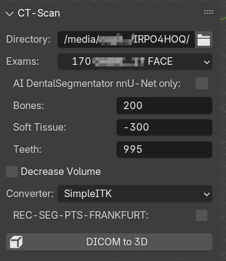
Fig. 58 Exam selected and ready to be reconstructed.
Once the desired exam is selected, the system searches the database for tomographs and configurations and adjusts the values of the factors; in this case, Bones: 200, Soft Tissue: -300, and Teeth: 995. If the user chooses to reconstruct only these three 3D meshes, they could already do so, but to generate the composite skull and leverage the segmentations via artificial intelligence, an extra step is required (Fig. 58).
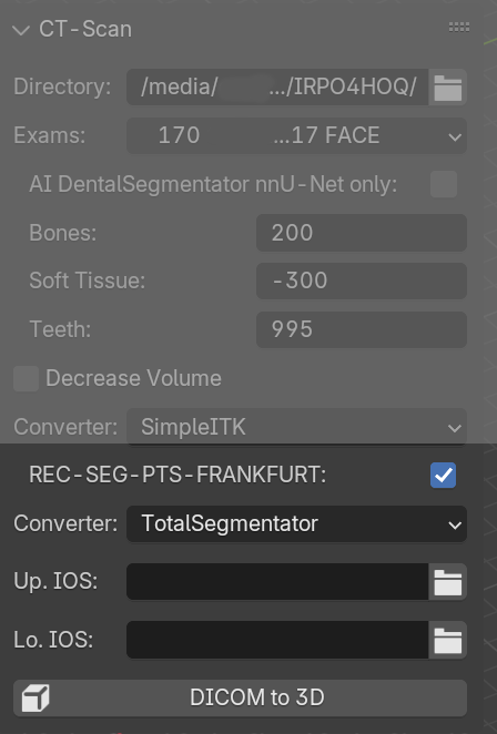
Fig. 59 REC-SEG-PTS-FRANKFURT activated; the lighter coloring above was made solely to highlight the region of interest.
This step consists of activating the REC-SEG-PTS-FRANKFURT checkbox, which now, by default, already activates the TotalSegmentator option. Here, the user can also proceed with the reconstruction if desired, but if the goal is to generate the composite skull, it is necessary to specify where the scanned intraoral models (IOS) are located. To do this, the user must click on the icon representing the model in question, such as Up. IOS (Fig. 59).
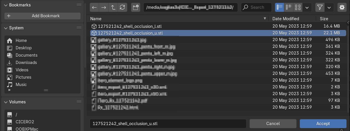
Fig. 60 Selection of the upper intraoral model.
Once this is done, simply click on the STL file corresponding to the upper model and then press the Accept button (Fig. 60).
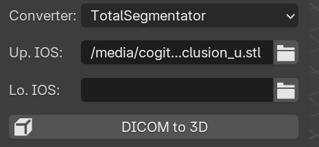
Fig. 61 Upper model set.
Thus, its location will be set in the interface (Fig. 61). Now it is the turn of the lower model, Lo. IOS.
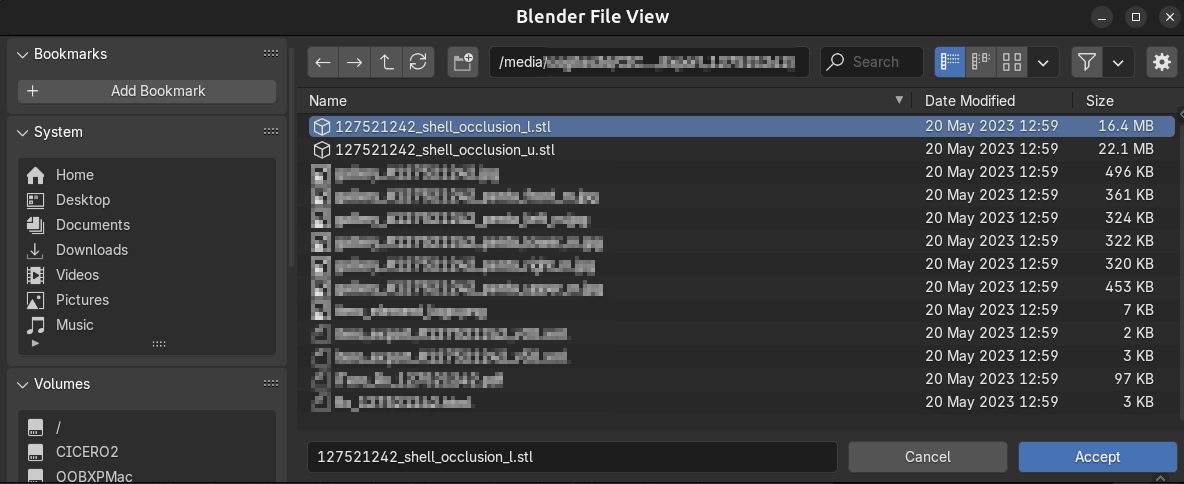
Fig. 62 Selection of the lower model.
This time, the lower model is selected (Fig. 62).
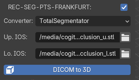
Fig. 63 Models selected and reconstruction initiated.
With the exam, configuration, and file paths provided, the unified reconstruction can be started by clicking on DICOM to 3D (Fig. 63).
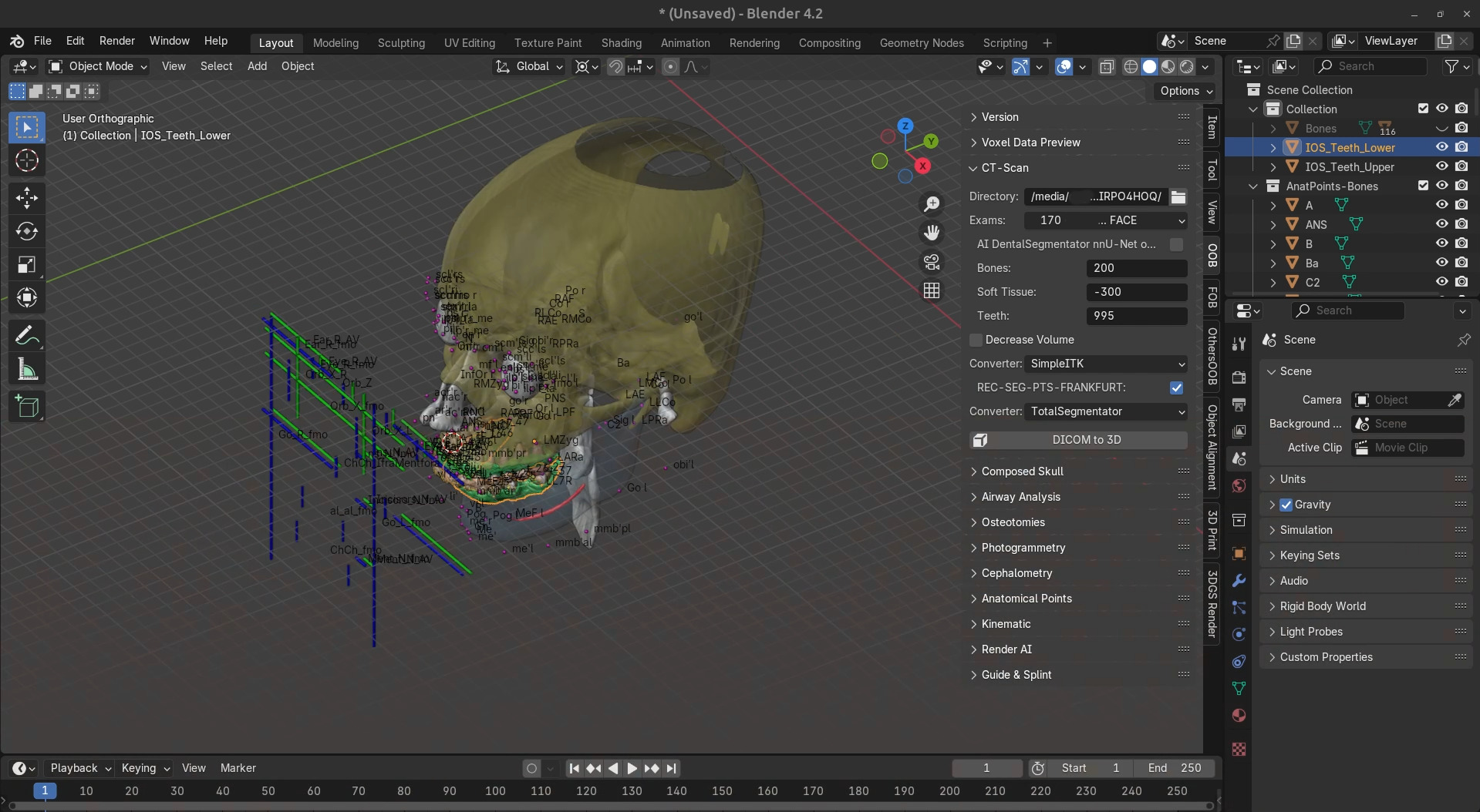
Fig. 64 Resulting meshes and data.
After a few minutes, depending on the GPU model, the reconstructed data is updated in the 3D scene (Fig. 64).
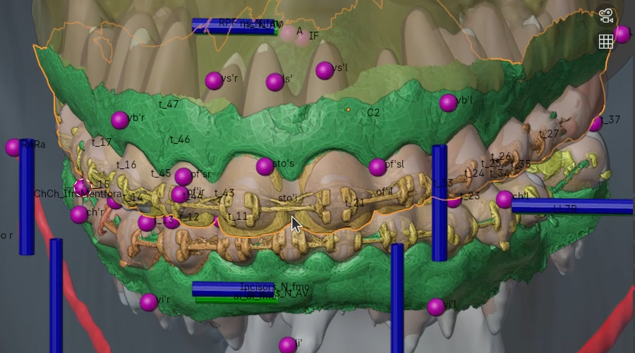
Fig. 65 Intraoral models automatically segmented and aligned.
One of the most evident new features of this version is the precise automatic segmentation and alignment of intraoral models (Fig. 65).
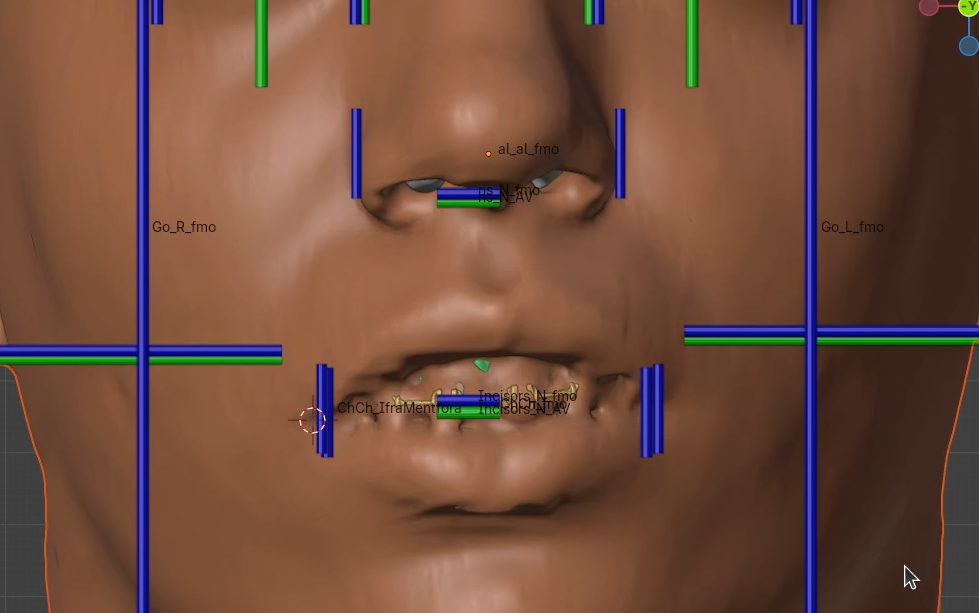
Fig. 66 Facial and skull projections.
Furthermore, a series of markings related to the expected boundaries for some facial and skull regions can be observed. The image demonstrates that the lip boundaries and nasal wings proposed by the algorithm are compatible with those of the face, even though the approaches are independent (Fig. 66).
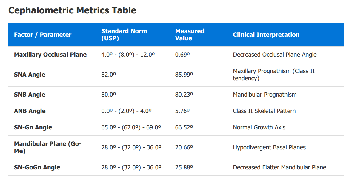
Fig. 67 USP cephalometry report.
Thanks to the individual placement of landmarks on the teeth, it is possible to generate the USP cephalometry report directly from the tomography reconstruction stage (Fig. 67). The Arnett cephalometry is also currently being ported/adapted to OOB XP.
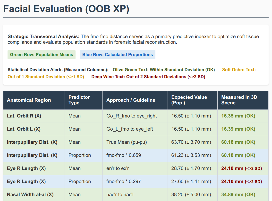
Fig. 68 Report of facial measurements versus population data.
The provision of anatomical landmarks, both on bones and soft tissue, also enabled the generation of a report for the patient’s facial measurements, comparing them with the population data available in OOB XP. This report allows the surgeon to observe the patient’s structure in relation not only to the population mean but also to proportion-based projections (Fig. 68).
Testing and Best Practices
The previous step-by-step section addressed only the tool in its operational state, after undergoing a series of tests and adjustments. Some points related to this stage will be discussed below.
Information about the computer used: Intel Core i9 9900K 3.6 GHz/16M processor; 64 GB of RAM; GeForce 8 GB GDDR6 256-bit RTX 2070 GPU; Gigabyte 1151 Z390 motherboard; SSD SATA III 960 GB 2.5”; SSD SATA III 480 GB 2.5”; Masterliquid 240V Water Cooler; Linux Ubuntu 24.04 and Windows 11.
An important point to note regarding AI-driven CT-Scan segmentation tools is that they only function if the orientation of the DICOM files is axial; otherwise, they will not perform their task. On the other hand, MeshSegNet, which is related to tooth segmentation, proved to be highly robust and functioned even with orientations in different axes.
ID |
Time (s) |
Failures |
Brackets |
Axis |
|---|---|---|---|---|
1 |
28 |
1 |
no |
Z |
2 |
34 |
1 |
yes |
Z |
3 |
23 |
0 |
yes |
Z |
4 |
22 |
0 |
no |
Z |
5 |
20 |
2 |
no |
X |
6 |
23 |
3 |
yes |
Z |
7 |
22 |
1 |
yes |
Z |
8 |
24 |
1 |
yes |
Z |
9 |
35 |
4 |
yes |
Z |
10 |
22 |
0 |
yes |
Z |
11 |
20 |
0 |
no |
Z |
12 |
23 |
2 |
no |
Y |
13 |
23 |
0 |
yes |
X |
14 |
24 |
4 |
yes |
Z |
15 |
25 |
0 |
yes |
Y |
16 |
24 |
0 |
yes |
Y |
17 |
20 |
0 |
yes |
Z |
18 |
21 |
1 |
yes |
Z |
19 |
24 |
0 |
yes |
Y |
20 |
32 |
2 |
yes |
X/Y/Z |
21 |
19 |
0 |
no |
X |
22 |
21 |
1 |
yes |
Z |
23 |
23 |
0 |
no |
Y |
24 |
24 |
2 |
no |
Y |
Average |
24 |
1 |
In an initial test with 24 dental arch pairs (24 upper and 24 lower), tooth recognition remained significantly stable, even when dealing with orientations in different axes. The average time for the segmentation of two dental arches was 24 seconds on the PC used, and the average error rate was just 1 unmarked tooth (Table 1).
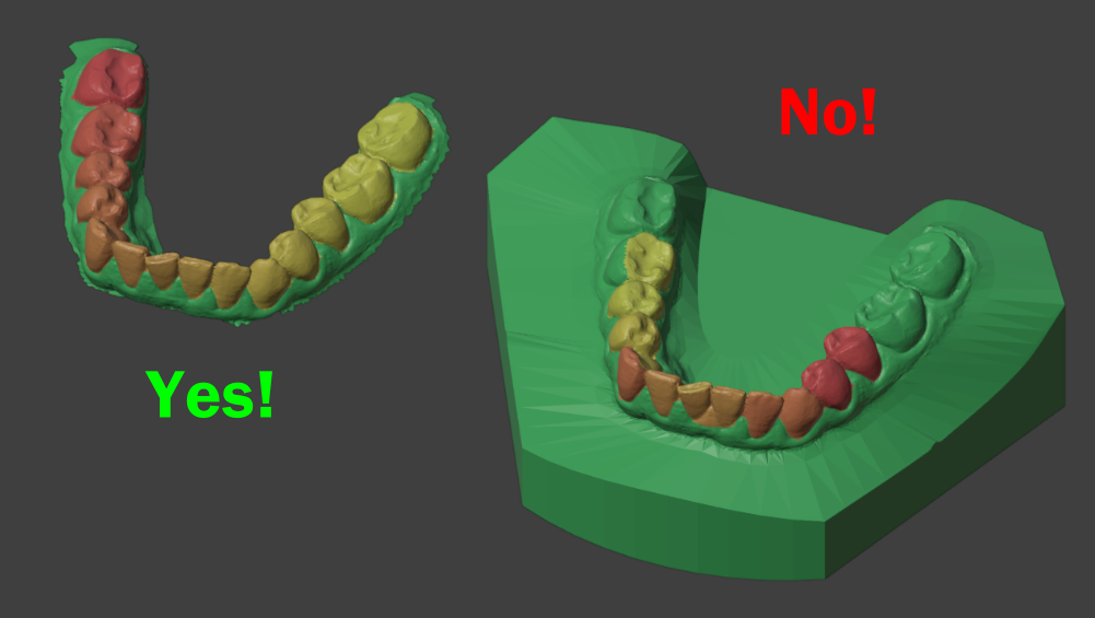
Fig. 69 Quality difference between isolated teeth and the model mounted for printing.
The tests were expanded to include models mounted for printing. These models typically generate a considerably higher number of errors, often ignoring several teeth or partially recognizing only a small portion of them. By isolating the gingiva and the teeth, the segmentation result improves significantly (Fig. 69).
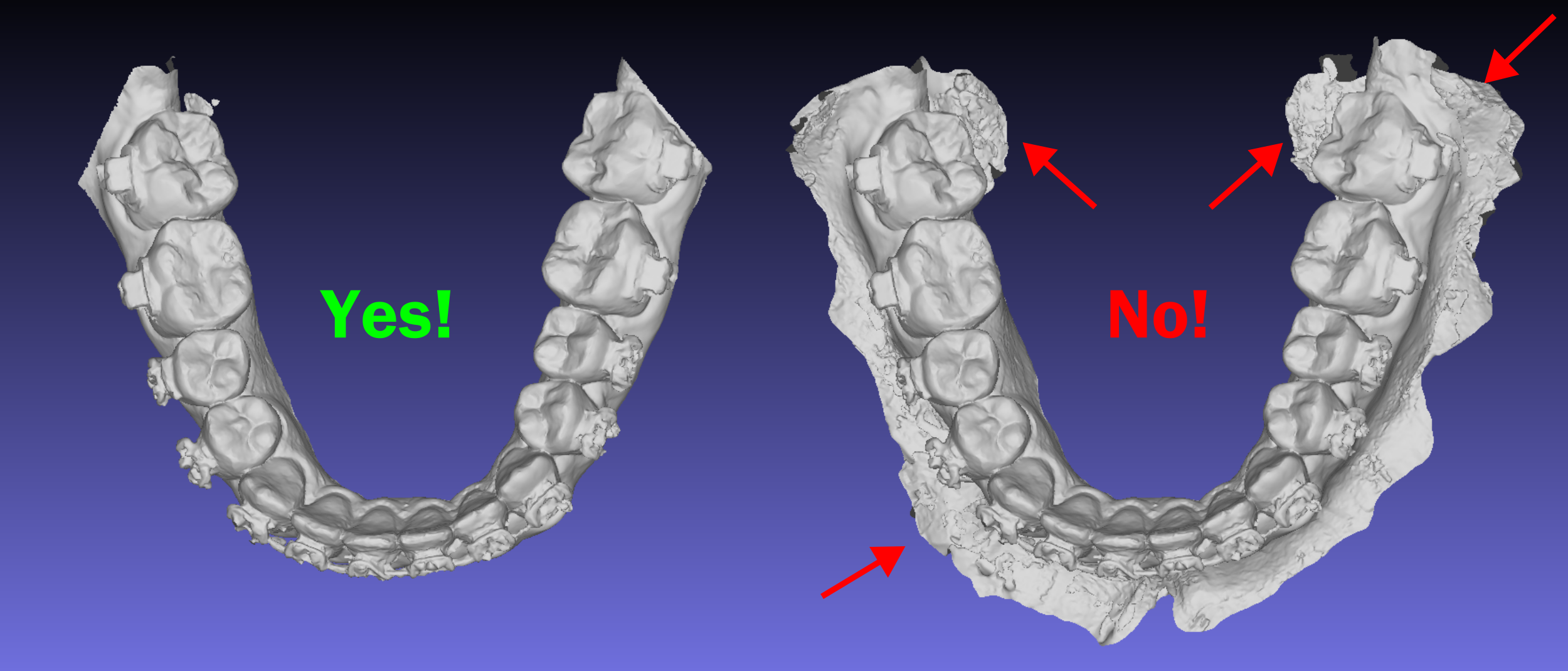
Fig. 70 Intraoral scan with surface noise.
Subsequently, issues related to areas with digitization noise were also identified (Fig. 70), thereby showing that a good practice is to avoid using models mounted in the pipeline or those with excessive noise. It is expected that intraoral models are composed solely of teeth and the jaw in a single-wall mesh, without thickness—such as some scanners might generate when focusing on subsequent 3D printing.
Another test consisted of selecting 23 complete exams, containing computed tomography scans and intraoral models, and running the composite skull generation system under both Linux (Ubuntu 24.04) and Windows 11. The outcomes corroborated the testing history (see Introduction references), where Linux is generally faster than Windows in executing tasks. What caused some concern was that, despite involving the exact same tools and generally identical library versions, errors under Windows are higher. This is evident as one of the tomographies failed to process on that system and alignment errors were double: 6 vs. 3. After the first round of testing, some programming adjustments were implemented, and the number of errors dropped drastically: under Linux it decreased from 3 to 1, and under Windows it fell from 6 to 3 (Table 2).
ID |
Linux Time (m:s) |
Linux Errors |
Windows Time (m:s) |
Windows Errors |
|---|---|---|---|---|
1 |
09:21 |
0 |
18:15 |
0 |
2 |
08:21 |
0 |
13:26 |
0 |
3 |
08:46 |
0 |
16:15 |
0 |
4 |
07:57 |
0 |
13:57 |
0 |
5 |
08:38 |
0 |
13:50 |
0 |
6 |
08:56 |
0 |
14:25 |
0 |
7 |
08:58 |
1 |
13:41 |
1 |
8 |
09:56 |
0 |
15:35 |
1 |
9 |
10:09 |
0 |
15:47 |
1 |
10 |
09:50 |
0 |
15:04 |
0 |
11 |
17:10 |
0 |
18:51 |
0 |
12 |
09:34 |
0 |
16:23 |
0 |
13 |
08:44 |
0 |
13:36 |
0 |
14 |
08:49 |
0 |
- |
- |
15 |
10:10 |
0 |
13:39 |
0 |
16 |
09:47 |
1 (fix.) |
13:41 |
1 (fix.) |
17 |
08:46 |
0 |
12:21 |
0 |
18 |
11:03 |
0 |
15:18 |
0 |
19 |
15:22 |
0 |
22:03 |
0 |
20 |
07:57 |
0 |
12:20 |
0 |
21 |
13:44 |
1 (fix.) |
20:11 |
1 (fix.) |
22 |
22:49 |
0 |
27:11 |
0 |
23 |
12:23 |
0 |
17:13 |
1 (fix.) |
Before (Average) |
10:45 |
3/46 |
16:03 |
6/44 |
Post-Corrections |
1/46 |
3/44 |
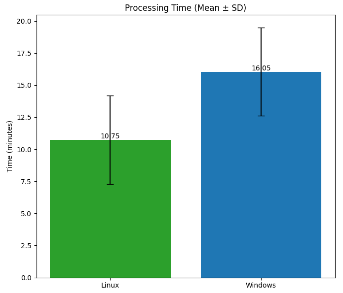
Fig. 71 Comparison between processing times (seconds converted into decimals).
Even though the time factor showed a significant difference, 10.75 minutes vs. 16.05 minutes (Fig. 71), the standard deviations overlapped. There is a curious behavior in AI segmentation workflows, where processing can take longer the first time it is executed, followed by a downward trend in duration. Furthermore, the same exam does not always require the same processing time, and substantial variations can occur. The precise mechanism responsible for this was not studied in depth, but this reality does not compromise the results, which are the most critical element of the approach.
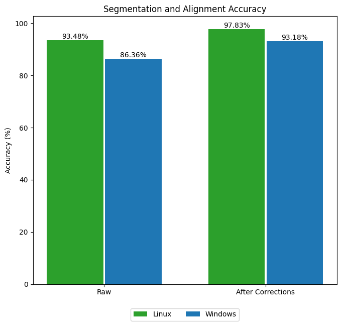
Fig. 72 Comparison between accuracy.
Looking specifically at the automatic alignment of intraoral models, the first raw run showed 3 error occurrences out of 46 arches under Linux, yielding a 6.52% error rate (93.48% accuracy). Under Windows, there were 6 occurrences out of 44 arches (as one exam failed completely), resulting in a 13.64% error rate (86.36% accuracy). After the code adjustment, errors decreased significantly: Linux dropped to just 1 error (97.83% accuracy), while Windows dropped to 3 errors (93.18% accuracy).
However, while these arch-isolated metrics look highly promising, clinical diagnostics dictate that there is no such thing as a “half-error.” If either arch fails to align properly, the global context of the exam is compromised. Adjusting the post-correction results to reflect complete patient exams, Linux presented 1 error out of 23 exams, achieving an accuracy of 95.65%. Conversely, Windows presented 3 failed exams out of 22 valid ones (roughly 1 error every 7 exams), limiting its accuracy to 86.36%. At this level, when isolating the residual failure rate alone, Linux proves to be approximately 3 times more effective than Windows regarding automated alignment accuracy.
Having compared the same approach across different operating systems, the next step was to compare the 23 composite skull configurations between TotalSegmentator+MeshSegNet and DentalSegmentator. Running the same 23 exams yielded striking results, as the processing time alone revealed a significant difference: 10m45s for the former against 20m25s for the DentalSegmentator. Regarding alignment, the disparity was even wider, presenting only 1 error out of 46 arches (97.83%), or 1 out of 23 patients (95.65% accuracy) for TotalSegmentator, compared to 31 errors out of 46 arches (32.61% accuracy) or 22 failed exams out of 23 patients (leaving a mere 4.35% global accuracy) for DentalSegmentator (Table 3). When analyzing global patient success alone, the difference between the two approaches is glaring, proving that the new TotalSegmentator+MeshSegNet pipeline is approximately 22 times more accurate than the DentalSegmentator.
ID |
TotalSeg Time |
TotalSeg Err |
DentalSeg Time |
DentalSeg Err |
|---|---|---|---|---|
1 |
09:21 |
0 |
10:27 |
1 |
2 |
08:21 |
0 |
13:14 |
2 |
3 |
08:46 |
0 |
11:08 |
1 |
4 |
07:57 |
0 |
09:50 |
1 |
5 |
08:38 |
0 |
11:14 |
1 |
6 |
08:56 |
0 |
24:45 |
1 |
7 |
08:58 |
1 |
19:57 |
2 |
8 |
09:56 |
0 |
28:35 |
2 |
9 |
10:09 |
0 |
19:37 |
0 |
10 |
09:50 |
0 |
11:18 |
1 |
11 |
17:10 |
0 |
35:49 |
1 |
12 |
09:34 |
0 |
13:47 |
2 |
13 |
08:44 |
0 |
12:44 |
2 |
14 |
08:49 |
0 |
17:46 |
1 |
15 |
10:10 |
0 |
35:02 |
2 |
16 |
09:47 |
0 |
31:09 |
1 |
17 |
08:46 |
0 |
31:11 |
2 |
18 |
11:03 |
0 |
24:28 |
1 |
19 |
15:22 |
0 |
28:23 |
1 |
20 |
07:57 |
0 |
08:22 |
2 |
21 |
13:44 |
0 |
24:50 |
1 |
22 |
22:49 |
0 |
15:58 |
2 |
23 |
12:23 |
0 |
30:11 |
1 |
Avg. |
10:45 |
20:25 |
||
Total |
1/46 |
31/46 |
This outcome does not imply that either method is invalid, since both workflows still allow manual rotation or isolated ICP adjustments to refine intraoral model alignment. The advantage of TotalSegmentator in this scenario relies on two factors: first, it segmentates teeth individually, enabling OOB XP to capture landmarks that will subsequently align with MeshSegNet tooth segmentation outputs on the intraoral model. Even if potential inaccuracies exist in both approaches, data and procedural redundancy help fill these gaps, resulting in a fully aligned model—the ultimate goal of the unified composite skull system. Furthermore, another factor favors TotalSegmentator: while it segmentates a total of 74 anatomical structures, from which OOB XP filters 49 (though some might be missing, such as third molars), DentalSegmentator provides only 5 segmentations and takes nearly twice as long, even without counting the MeshSegNet segmentation phase included in the competing pipeline. This performance gap, combined with minor quality discrepancies observed between models generated in Linux and Windows, was decisive in choosing TotalSegmentator as the default framework. Nevertheless, given its robustness and proven validation, DentalSegmentator will remain available, providing users with an alternative option for structural validation whenever required, as discussed below.
ID |
Linux Time (m:s) |
Linux Errors |
ID |
Linux Time (m:s) |
Linux Errors |
|---|---|---|---|---|---|
24 |
07:50 |
0 |
43 |
09:37 |
0 |
25 |
07:47 |
0 |
44 |
10:37 |
0 |
26 |
09:49 |
0 |
45 |
09:19 |
1 |
27 |
10:59 |
0 |
46 |
12:26 |
0 |
28 |
10:20 |
0 |
47 |
14:04 |
0 |
29 |
10:20 |
0 |
48 |
08:48 |
1 |
30 |
07:54 |
0 |
49 |
08:48 |
0 |
31 |
09:20 |
0 |
50 |
10:22 |
0 |
32 |
07:25 |
0 |
51 |
08:51 |
0 |
33 |
10:54 |
0 |
52 |
22:29 |
0 |
34 |
12:36 |
0 |
53 |
11:34 |
0 |
35 |
08:48 |
0 |
54 |
10:00 |
0 |
36 |
14:06 |
0 |
55 |
21:57 |
0 |
37 |
08:10 |
0 |
56 |
22:05 |
0 |
38 |
07:01 |
0 |
57 |
12:19 |
0 |
39 |
08:03 |
0 |
58 |
10:27 |
0 |
40 |
14:19 |
0 |
59 |
10:10 |
0 |
41 |
08:29 |
0 |
60 |
23:46 |
0 |
42 |
08:23 |
0 |
Avg. |
11:07 |
|
Total |
3/120 |
An extension of the test was carried out, reaching a total of 60 cases and 120 arches. Within this expanded sample, the workflow presented only 3 errors out of 120 arches (97.50% accuracy), corresponding to 3 failed alignment outcomes out of 60 patient cases (95.00% global accuracy). Analysing the outliers individually, the model for ID 7 was found to be negatively rotated around the Z-axis by approximately 45° (pointing backwards and sideways) while presenting minor structural noise. Once this orientation was manually corrected, the arches aligned properly, revealing a slight spatial discrepancy between the intraoral scan teeth and those from the computed tomography (CT) scan. This phenomenon occurs naturally in clinical practice when there is a significant time gap between the CT acquisition and the intraoral scanning, during which physiological tooth movement may occur.
Conversely, case ID 45 involved a digital scan derived from a physical plaster model, displaying extrusion artifacts around orthodontic brackets and poor overall mesh quality—typical technical constraints that can compromise analogue-to-digital 3D orthodontic documentation. Meanwhile, case ID 48 offered no obvious explanation for the automated alignment failure, given that the scan exhibited high mesh quality and its initial orientation aligned perfectly with the patient’s standard axial position. These findings demonstrate that despite strictly following protocols, residual error margins persist, rendering the 95.00% global accuracy a highly significant milestone for the current version of the framework. Furthermore, it highlights that while the software drastically simplifies and accelerates the clinician’s workflow, it relies on professional oversight and visual validation at every stage, adding a crucial layer of human security to the clinical digital pipeline.
Statistical Treatment Results
Inferential analysis confirmed significant advantages in the technological infrastructure transition. The Wilcoxon signed-rank test demonstrated that processing time under the Linux platform (Mean = 10.75 min) is statistically shorter than in the Windows environment (Mean = 16.05 min) (\(p < .001\)). Similarly, the new pipeline based on TotalSegmentator+MeshSegNet (Mean = 10.75 min) drastically outperformed the legacy DentalSegmentator tool in speed (Mean = 20.42 min) (\(p < .001\)).
Regarding patient alignment accuracy in the initial comparative sample, Linux achieved a higher nominal rate than Windows (95.65%, 95% CI: [79.01%, 99.23%] vs. 86.36%, 95% CI: [66.67%, 95.25%]). However, McNemar’s paired test indicated that the difference in strict residual error frequencies between the operating systems did not reach formal statistical significance for this sample size (\(p = .250\)). In contrast, McNemar’s test confirmed the absolute superiority of the new pipeline compared to DentalSegmentator (4.35%, 95% CI: [0.77%, 20.99%]), with high statistical significance (\(p < .001\)).
In the large-scale expanded validation under the Linux environment involving 60 clinical cases (120 arches), the mathematical stability of the new ecosystem consolidated at high levels. The system achieved an accuracy of 97.50% for isolated arches (95% CI: [92.91%, 99.15%]). Under the global patient-level clinical criterion (success conditioned on the correct simultaneous alignment of both arches), the rate settled at 95.00% (95% CI: [86.30%, 98.29%]), narrowing the confidence intervals and validating the predictability and methodological robustness of the automation implemented in OrtogOnBlender XP.
Discussion
The composite skull generation system is created during what has been established as “passive working time,” where the user does not interact, waiting for the system to perform all configurations automatically. In its essence, it is a modular and redundant structure, as the same general anatomy is reconstructed and measured multiple times, allowing any reconstruction issue to become visible. This reduces the probability of structural errors, such as varied scales or unwanted structural mirroring.
Structural coherence is essential for a successful surgical planning process since any inconsistency in dimensions or anatomical reconstruction can not only compromise the calculated guides and approaches but also pose a risk to the patient. Historically, the OOB has relied on systems tested under stress to determine the confidence level of an anatomical reconstruction, such as the conversion of computed tomography scans into 3D meshes. The oldest system, which originated from DicomToSTL and was ported to VTK-ITK, was legacy, improved, and tested in OOB XP, as previously discussed; therefore, it constitutes an element present in the unified import system, as it serves the purpose of maintaining the main skull as a parenting base and pre-surgical reference, while providing the Soft Tissue for use in osteotomy simulations. The other systems “talk to each other” and reinforce validation in a cross-referenced manner, as will be seen below.
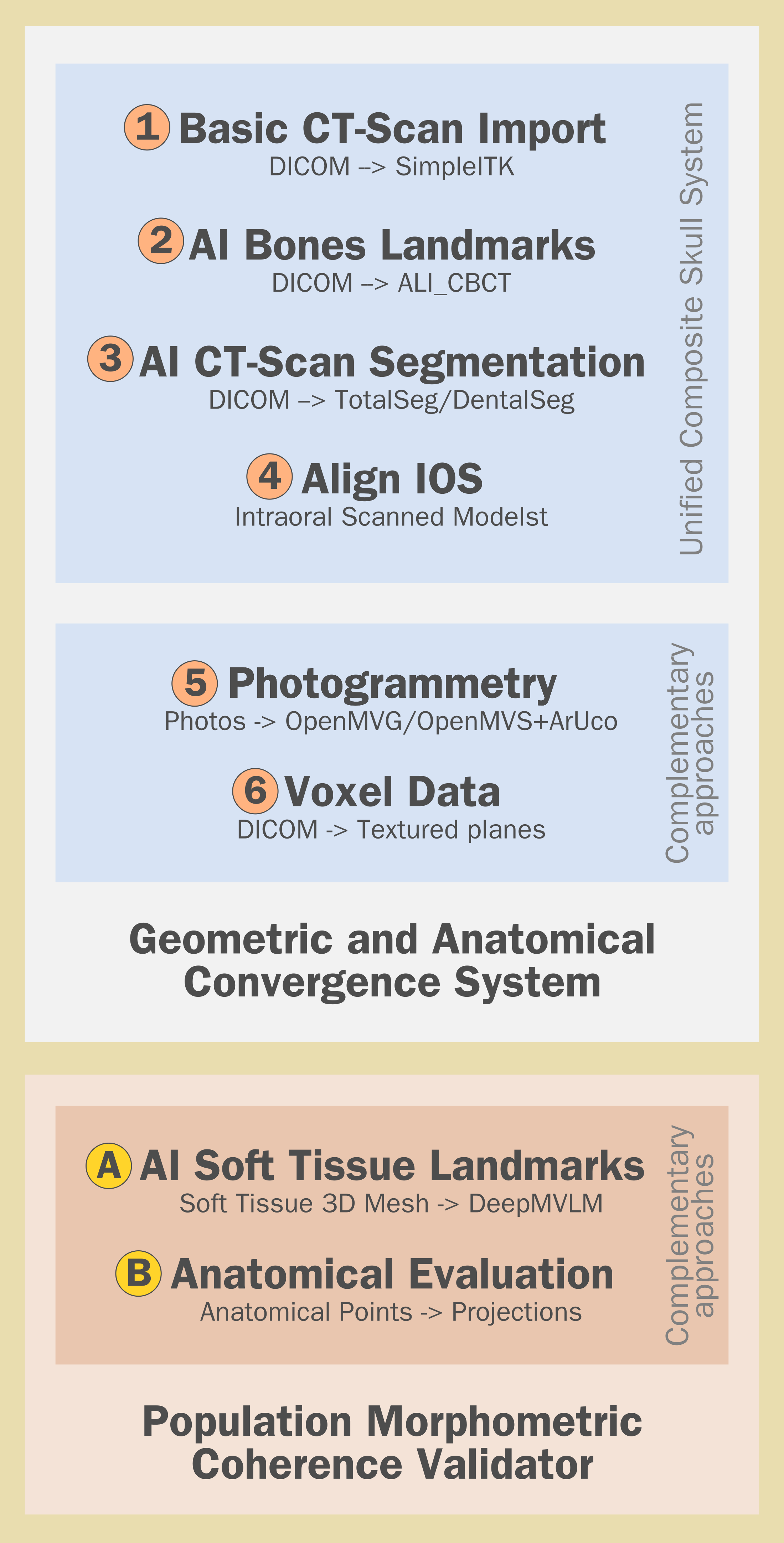
Fig. 73 Structural and anatomical validation scheme.
The most reliable base for reconstruction is the legacy system that generates three meshes: the skull (general bone), the soft tissue, and the teeth (hard tissue). The default library is SimpleITK, which pulls the data from the original DICOM for the reconstruction (Fig. 73, 1). Being an old and reliable system, it ends up serving as the general structural foundation. The anatomical landmark positioning system (Fig. 73, 2) acts as a structural validation system, as it utilizes a different approach—the ALI_CBCT solution—and if there is any inconsistency between the points and the reconstructed anatomy, it will become evident in the 3D scene. The segmentation tools also use different approaches, such as the standard TotalSegmentator and DentalSegmentator, both of which pull data from the original DICOM to reconstruct individual anatomies (Fig. 73, 3).
Finally, there is the alignment of intraoral models (IOS), which imports the file originating from the structured light scanning process—something entirely different from the previous reconstructions. Since it deals with smaller elements that require higher resolution, it serves to highlight inconsistencies in both scale and potential mirrorings in the previous reconstructions, adding an extra layer of confidence to the process (Fig. 73, 4). Thus, a cross-validation system with independent elements configured in four layers is established.
However, validations can be extended into two other layers: one performed by facial digitization via photogrammetry [Moraes_et_al_2025b_f], i.e., through photos and scaled by ArUco markers (Fig. 73, 5), which is entirely different from the other structures. And finally, the reconstruction of voxel data, which captures the DICOM slices, importing them into the spaces fixed by the file data and generating another visual element with a completely different approach (Fig. 73, 6). There is thus a system composed of six validation elements at our disposal, grouped into what is now called the Geometric and Anatomical Convergence System.
Two other complementary elements, though in a slightly different manner, are the soft tissue anatomical landmark positioner (Fig. 73, A), which works in conjunction with the bone landmark system, enabling the Anatomical Evaluation (Fig. 73, B) to generate not only the text report but also trigger the visual elements for expected boundaries and positioning for both soft tissue and bones. Even though it is not a direct validator of real anatomical measurements, by reporting the expected dimensions through means and proportions, it provides a reference for the expected structure, hence the name Population Morphometric Coherence Validator.
Conclusion
The automation of the unified composite skull import system in OrtogOnBlender XP represents a disruptive technological leap for maxillofacial surgical planning, transforming processes previously characterized by exhaustive manual segmentation into fluid, data-driven workflows. The consolidation of the new pipeline based on TotalSegmentator and MeshSegNet not only drastically optimized passive computational processing time to half of its previous duration, but also established an unprecedented global accuracy threshold of ~95% per patient, overcoming by more than 20 times the critical limitations observed in legacy tools such as DentalSegmentator.
The performance results reinforce that the choice of computational platform plays a critical role in the predictability of the digital routine, demonstrating that the Linux environment remains considerably superior and approximately 3 times more resilient against residual alignment failures compared to the Windows ecosystem. Furthermore, the foundation of the Geometric and Anatomical Convergence System demonstrates that structured methodological redundancy in independent multilayers functions as a robust barrier against scale discrepancies and volumetric mirroring. Ultimately, while artificial intelligence masterfully assumes the operational complexity of 3D mesh engineering, the study reiterates that clinical judgment and the surgeon’s visual audit persist as the ultimate and irreplaceable instances of biological security in the contemporary digital pipeline.
References
Abdullah, J. Y., Moraes, C., Saidin, M., Rajion, Z. A., Hadi, H., Shahidan, S., & Abdullah, J. M. (2022). Forensic Facial Approximation of 5000-Year-Old Female Skull from Shell Midden in Guar Kepah, Malaysia. Applied Sciences, 12(15), 7871. https://doi.org/10.3390/app12157871
Moraes, C., Rosa, E. da, & Dornelles, R. (2020). Protocolo de Tomografia para Planejamento de Cirurgia Ortognática. figshare. https://doi.org/10.6084/M9.FIGSHARE.12923807
Moraes, C., Dornelles, R., & Rosa, E. da. (2021). Sistema de Reconstrução de Tomografia Computadorizada Baseado no Slicer 3D e no DicomToMesh. figshare. https://doi.org/10.6084/M9.FIGSHARE.13513890
Moraes, C., Dakir, I., Dornelles, R., & Rosa, E. da. (2021). Reconstrução de Tomografias com o VTK Python, o SimpleITK e o Multiprocessing. figshare. https://doi.org/10.6084/M9.FIGSHARE.14370902
Moraes, C., Schreiner, T., Startek, B., & Beaini, T. L. (2024). Alinhamento em Frankfurt, Colocação de Pontos Anatômicos e Segmentação do Crânio por Inteligência Artificial no OrtogOnBlender. figshare. https://doi.org/10.6084/M9.FIGSHARE.25140020
Moraes, C., Dakir, I., Startek, B., Dornelles, R., & Rosa, E. da. (2024). Ferramenta de Importação de Tomografia Computadorizada no OrtogOnBlender XP. figshare. https://doi.org/10.6084/M9.FIGSHARE.27648876
Moraes, C., Dakir, I., Startek, B., Dornelles, R., & Rosa, E. da. (2024). Segmentação de Tomografias Computadorizadas por IA no OrtogOnBlender XP. figshare. https://doi.org/10.6084/M9.FIGSHARE.27761970
Moraes, C., Startek, B., Dakir, I., Schreiner, T., Dornelles, R., & Rosa, E. da. (2025). Sistema Unificado para a Criação de um Crânio Composto no OrtogOnBlender XP. figshare. https://doi.org/10.6084/M9.FIGSHARE.28135760
Moraes, C., Moulon, P., Bezzi, A., Moura, L., Rosa, E., Dornelles, R., Bezzi, A. (2025). Photogrammetry in OrtogOnBlender XP: The Story of an (R)Evolution. figshare. https://doi.org/10.6084/M9.FIGSHARE.30656390
Moraes, C., & Suharschi, I. (2022). Mensuração de Dados Faciais Ortográficos em Moldavos e Comparação com Outras Populações. figshare. https://doi.org/10.6084/M9.FIGSHARE.20089754
Moraes, C., & Dakir, I. (2021). Segmentação Automática dos Dentes com o MeshSegNet e o OrtogOnBlender. figshare. https://doi.org/10.6084/M9.FIGSHARE.14850105
Wasserthal, J., Breit, H.-C., Meyer, M. T., Pradella, M., Hinck, D., Sauter, A. W., Heye, T., Boll, D. T., Cyriac, J., Yang, S., Bach, M., & Segeroth, M. (2023). TotalSegmentator: Robust Segmentation of 104 Anatomic Structures in CT Images. Radiology: Artificial Intelligence, 5(5). https://doi.org/10.1148/ryai.230024